Multivariate interrupted time series models#

One modeling approach we could use for causal analysis of product incrementality is the multivariate interrupted time series (MV-ITS) model. This model is a generalization of the interrupted time series model (ITS), which is a common approach in causal inference. The MV-ITS model allows us to estimate the causal impact of an intervention (e.g., a new product introduction) on multiple outcomes (e.g., sales of multiple products) simultaneously.

One of the differences between this model and the standard ITS modeling approach is that rather than having a binary off/on intervention, the time series of sales of the new product can be thought of as a graded intervention.

Building our intuition#

Below we outline the simplest possible version of the model to build up our intuition before we move on to more complex versions.

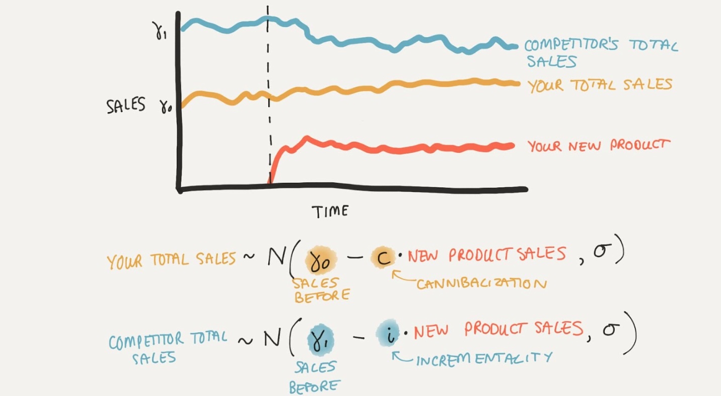
In this example we aggregate sales data into your companies total sales and your competitors total sales. We then have a time series of sales data for your company and your competitors. We can see that when we release a new product, our sales are not really affected, but our competitors’ total sales decrease. So an intuitively right answer here is that our new product has a high level of incrementality.

The MV-ITS approach

The MV-ITS approach models works as follows:

It models the time series of sales data for your company and your competitors.
These sales are modeled as normally distributed around an expected value with some degree of observation noise.
The model expectation could be built up of multiple components, such as a trend, seasonality, and the impact of marketing campaigns. However for this simple example we have an intercept only model.
Importantly, the expectation described above is decreased by some fraction of the new product sales. This fraction (across multiple sales outcomes) determines where the sales of the new product are coming from. From this, we can work out the level of incrementality of the new product.

The simplest saturated market model#

Let’s start with the simplest case:

The model description below assumes a saturated market. That is, new product sales have to be taken from existing sales and there is no growth of the overal size of the market.
We operate on aggregated sales data in that we have total sales for all your products and all your competitors products. We also have all the sales data for the new product that you released.

We’ll start by defining the model likelihood terms:

\[\begin{split} \begin{aligned} \vec{sales}_{your} \sim & \mathrm{Normal}(\gamma_{your} - c \cdot \vec{sales}_{new}, \sigma_{your})\\ \vec{sales}_{comp} \sim & \mathrm{Normal}(\gamma_{comp} - (1-c) \cdot \vec{sales}_{new}, \sigma_{comp}) \end{aligned} \end{split}\]

where \(\vec{sales}_{your}\), \(\vec{sales}_{comp}\), and \(\vec{sales}_{new}\) are the observed time series of sales of all your products, your competitors products, and your new product, respectively.

The parameter \(c \in [0, 1]\) is the proportion of new product sales that are cannibalistic, that is, have been taken from your existing products. Then \(1-c\) is the proportion of new product sales that are incremental, that is, have been taken from your competitors products. We can place a Beta prior on \(c\) to reflect our prior beliefs about the level of incrementality of the new product for example

The parameters \(\sigma_{your}\) and \(\sigma_{comp}\) are the standard deviations of the observation noise for your sales and your competitors sales, respectively. We can also place priors on these parameters to reflect our prior beliefs about the level of noise in the data.

This leaves the terms \(\gamma_{your}\) and \(\gamma_{comp}\), which are terms that model the sales of your products and your competitors products in the absence of the new product (which from a causal perspective we could also call the ‘intervention’). One way to think about this would be to construct a model for sales prior to the new product release. This could be a simple model with an intercept term, or a more complex model with trend and seasonality terms. Right now we will just use an intercept term to keep things simple in this first model. In this case \(\gamma_{your}\) and \(\gamma_{comp}\) are simply parameters, intercept terms for your sales and your competitors sales, respectively. Again, we can place priors on these parameters to reflect our prior beliefs about the level of sales in the absence of the new product, but the exact form is not crucial at this point.

Modelling products#

We could relax one of the simplifications - rather than model aggregated sales for your or your competitors products, we could model sales for each product individually. This would allow us to see which products are most affected by the new product release. We could write the new likelihood terms as:

\[\begin{split} \begin{aligned} \vec{sales}_1 \sim & \mathrm{Normal}(\gamma_1 - \beta_1 \cdot \vec{sales}_{new}, \sigma_1)\\ \vec{sales}_2 \sim & \mathrm{Normal}(\gamma_2 - \beta_2 \cdot \vec{sales}_{new}, \sigma_2)\\ \vdots \\ \vec{sales}_P \sim & \mathrm{Normal}(\gamma_P - \beta_P \cdot \vec{sales}_{new}, \sigma_P) \end{aligned} \end{split}\]

So now we have products \(p=1, \ldots, P\) and we could model the sales of each product individually. We now have a new parameter \(\beta_i\) for each product, which is the proportion of new product sales that are cannibalistic for that product. This allows us to see which products are most affected by the new product release. Because we have the assumption that the market is saturated, we can see that the sum of the \(\beta_i\)’s should equal 1. So it might be natural to place a Dirichlet prior on the \(\beta_i\)’s:

\[ \beta_1, \beta_2, \ldots, \beta_P \sim \mathrm{Dirichlet}(\alpha_1, \ldots, \alpha_P) \]

where all the \(\alpha\) hyperparameters could be 1, for example.

As long as we have a list of which products are your products and which are your competitors products, we can simply sum the approriate \(\beta_i\)’s to get the cannibalistic and incremental sales for your products and your competitors products.

The multivariate normal form

Note that you could re-write this model equivalently as:

\[\begin{split} \begin{bmatrix} \vec{sales}_1 \\ \vec{sales}_2 \\ \vdots \\ \vec{sales}_P \end{bmatrix} \sim \mathrm{MultivariateNormal}\left( \begin{bmatrix} \gamma_{1} - \beta_1 \cdot \vec{sales}_{new} \\ \gamma_{2} - \beta_2 \cdot \vec{sales}_{new} \\ \vdots \\ \gamma_{P} - \beta_P \cdot \vec{sales}_{new} \end{bmatrix}, \Sigma \right) \end{split}\]

We can embody the assumption that all the product sales are independent of each other by setting the off-diagonal elements of the covariance matrix \(\Sigma\) to zero. The diagonal elements of the covariance matrix are the variances of the observation noise for each product \([ \sigma_1, \sigma_2 \ldots, \sigma_P ]\). So the covariance matrix would look like:

\[\begin{split} \Sigma = \begin{pmatrix} \sigma_{1}^2 & 0 & \cdots & 0 \\ 0 & \sigma_{2}^2 & \cdots & 0 \\ \vdots & \vdots & \ddots & \vdots \\ 0 & 0 & \cdots & \sigma_{P}^2 \end{pmatrix} \end{split}\]

Relaxing independence assumptions#

We could relax the assumption that the sales of your products and your competitors products are independent. We could model the sales of your products and your competitors products as a multivariate normal distribution (see box above).

The key difference would be to additionally estimate the off-diagnal elements of the covariance matrix. This would allow us to model the correlation between the sales of all products. This might require us to put more work in to specifying the prior on the covariance matrix, but in some situations the benefits of this approach could be worth it. The covariance matrix would now look like:

\[\begin{split} \Sigma = \begin{pmatrix} \sigma_{11}^2 & \sigma_{12} & \cdots & \sigma_{1P} \\ \sigma_{21} & \sigma_{22}^2 & \cdots & \sigma_{2P} \\ \vdots & \vdots & \ddots & \vdots \\ \sigma_{P1} & \sigma_{P2} & \cdots & \sigma_{PP}^2 \end{pmatrix} \end{split}\]

The disadvantage of this model is that we would have a lot of parameters to estimate. For example, if there are \(P\) products then we could have to estimate \(P\) \(\beta_i\)’s and \(P\) standard deviations and \(P(P-1)/2\) covariances. This need not be a problem - we could place hierarchical priors on the \(\beta_i\)’s and the standard deviations for example, but it could be problematic with the covariances if we have a large number of products.

Moving to an unsaturated market#

Thus far we have considered the market as saturated. That is, it is assumed that the total sales of existing products are reduced by the same amount as the sales of the new product.

We could relax this assumption and consider an unsaturated market. More specifically, we could model the reduction of sales of existing products is less than the sales of the new product. Putting that another way, introduction of a new product leads to a reduction in existing product sales but there are additional sales of the new product which do not come from a reduction in the sales of existing products.

This requires only a minor change to the multivariate normal form of the model.

Specifically, rather than having \(P\) products which are the source of new product sales, we could simply add a psuedo-product which represents new sales. The first \(P\) products are as normal, all the existing products. The final pseudo product would represent the market growth. We could simply add an additional \(\beta\) parameter and specify the prior as:

\[ \beta_1, \beta_2, \ldots, \beta_P, \beta_{P+1} \sim \mathrm{Dirichlet}(\alpha_1, \ldots, \alpha_P, \alpha_{P+1}) \]

The rest of the model remains unchanged.

Previously the sum of the \(\beta\) parameters would be 1, which means that all new product sales are taken from existing products. Now the sum of the \(\beta\) parameters relating to existing products (\(\beta_1, \beta_2, \ldots, \beta_P\)) could be less than 1. When \(\beta_{P+1}>0\) then it means that the new product has caused the market to grow - some of the new product sales not come from reductions in sales of existing products.