Model deployment#

One of the main goals of PyMC-Marketing is to facilitate the deployment of its models.

This is achieved by building our models on top of ModelBuilder that offers a scikit-learn-like API and makes PyMC models easy to deploy.

PyMC-marketing models inherit 2 easy-to-use methods: save and load that can be used after the model has been fitted. All models can be configured with two standard dictionaries: model_config and sampler_config that are serialized during save and persisted after load, allowing model reuse across workflows.

We will illustrate this functionality with the example model described in the MMM Example Notebook. For sake of generality, we ommit most technical details here.

import arviz as az
import matplotlib.pyplot as plt
import numpy as np
import pandas as pd

from pymc_marketing.mmm import MMM, GeometricAdstock, LogisticSaturation
from pymc_marketing.prior import Prior

az.style.use("arviz-darkgrid")
plt.rcParams["figure.figsize"] = [12, 7]
plt.rcParams["figure.dpi"] = 100

%config InlineBackend.figure_format = "retina"

seed = sum(map(ord, "mmm"))
rng = np.random.default_rng(seed=seed)

Let’s load the dataset:

url = "https://raw.githubusercontent.com/pymc-labs/pymc-marketing/main/data/mmm_example.csv"
df = pd.read_csv(url, parse_dates=["date_week"])

columns_to_keep = [
    "date_week",
    "y",
    "x1",
    "x2",
    "event_1",
    "event_2",
    "dayofyear",
]

data = df[columns_to_keep].copy()
data["t"] = np.arange(df.shape[0])
data.head()

	date_week	y	x1	dayofyear	t
0	2018-04-02	3984.662237	0.318580	92	0
1	2018-04-09	3762.871794	0.112388	99	1
2	2018-04-16	4466.967388	0.292400	106	2
3	2018-04-23	3864.219373	0.071399	113	3
4	2018-04-30	4441.625278	0.386745	120	4

But for our model we need much smaller dataset, many of the previous features were contributing to generation of others, now as our target variable is computed we can filter out not needed columns:

Model and sampling configuration#

Model configuration#

We first illustrate the use of model_config to define custom priors within the model.

Because there are potentially many variables that can be configured, each model provides a default_model_config attribute. This will allow you to see which settings are available by default and only define the ones you need to change.

We need to create a dummy model to be able to see the configuration dictionary.

adstock = GeometricAdstock(l_max=8)
saturation = LogisticSaturation()

dummy_model = MMM(
    date_column="date_week",
    channel_columns=["x1", "x2"],
    adstock=adstock,
    saturation=saturation,
    control_columns=[
        "event_1",
        "event_2",
        "t",
    ],
    yearly_seasonality=2,
)
dummy_model.default_model_config

{'intercept': Prior("Normal", mu=0, sigma=2),
 'likelihood': Prior("Normal", sigma=Prior("HalfNormal", sigma=2)),
 'gamma_control': Prior("Normal", mu=0, sigma=2, dims="control"),
 'gamma_fourier': Prior("Laplace", mu=0, b=1, dims="fourier_mode"),
 'adstock_alpha': Prior("Beta", alpha=1, beta=3, dims="channel"),
 'saturation_lam': Prior("Gamma", alpha=3, beta=1, dims="channel"),
 'saturation_beta': Prior("HalfNormal", sigma=2, dims="channel")}

We can change the parameters that go into the distribution of each term. In this case we’ll just simply replace the sigma for saturation_beta with a custom one:

n_channels = 2

total_spend_per_channel = data[["x1", "x2"]].sum(axis=0)
spend_share = total_spend_per_channel / total_spend_per_channel.sum()

# The scale necessary to make a HalfNormal distribution have unit variance
HALFNORMAL_SCALE = 1 / np.sqrt(1 - 2 / np.pi)
prior_sigma = HALFNORMAL_SCALE * n_channels * spend_share.to_numpy()
prior_sigma

array([2.1775326 , 1.14026088])

saturation_beta = Prior("HalfNormal", sigma=prior_sigma, dims="channel")
my_model_config = {"saturation_beta": saturation_beta}

my_model_config

{'saturation_beta': Prior("HalfNormal", sigma=[2.1775326  1.14026088], dims="channel")}

As mentioned in the original notebook: “For the prior specification there is no right or wrong answer. It all depends on the data, the context and the assumptions you are willing to make. It is always recommended to do some prior predictive sampling and sensitivity analysis to check the impact of the priors on the posterior. We skip this here for the sake of simplicity. If you are not sure about specific priors, the MMM class has some default priors that you can use as a starting point.”

Sampling configuration#

The second feature we can customize is sampler_config. Similar to model_config, it’s a dictionary that gets saved and contains things you would usually pass to the fit() kwargs. It’s not mandatory to create your own sampler_config. The default MMM.sampler_config is empty because the default sampling parameters usually prove sufficient for a start.

dummy_model.default_sampler_config

{}

my_sampler_config = {
    "tune": 1000,
    "draws": 1000,
    "chains": 4,
    "target_accept": 0.91,
    "nuts_sampler": "numpyro",
}

Let’s finally assemble our model!

mmm = MMM(
    model_config=my_model_config,
    sampler_config=my_sampler_config,
    date_column="date_week",
    channel_columns=["x1", "x2"],
    adstock=adstock,
    saturation=saturation,
    control_columns=[
        "event_1",
        "event_2",
        "t",
    ],
    yearly_seasonality=2,
)

We can confirm our settings are being used

mmm.model_config["saturation_beta"]

Prior("HalfNormal", sigma=[2.1775326  1.14026088], dims="channel")

mmm.sampler_config

{'tune': 1000,
 'draws': 1000,
 'chains': 4,
 'target_accept': 0.91,
 'nuts_sampler': 'numpyro'}

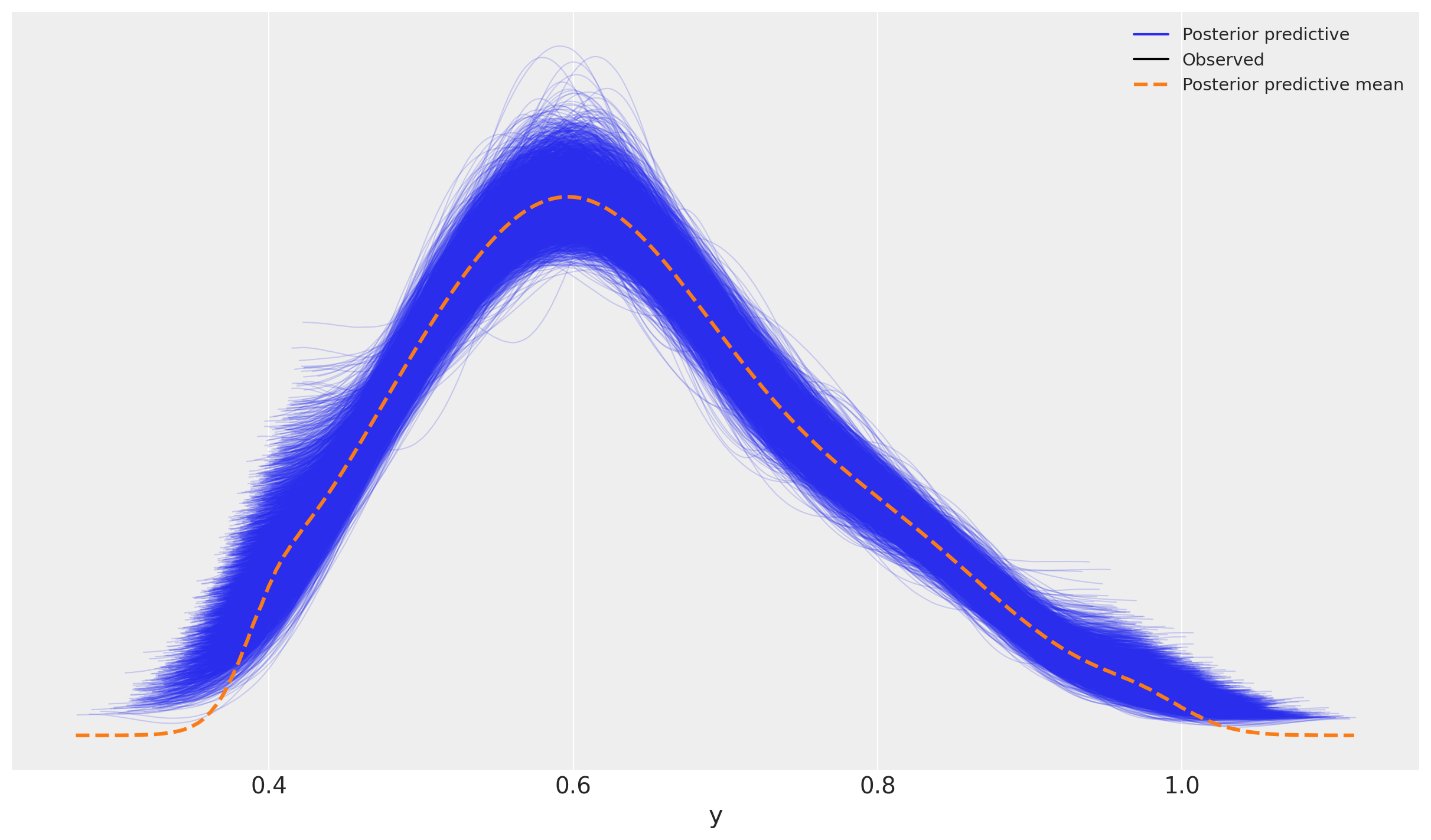
Other models#

Even though this introduction is using MMM, all other PyMC-Marketing models (MMM and CLV) provide these functionalities as well.

Summary#

The PyMC-Marketing functionalities described here are intended to facilitate model sharing among data science teams without demanding extensive modelling technical knowledge for everyone involved. We are still iterating on our API and would love to hear more feedback from our users!

%load_ext watermark
%watermark -n -u -v -iv -w -p pytensor

Last updated: Thu Nov 14 2024

Python implementation: CPython
Python version       : 3.12.4
IPython version      : 8.27.0

pytensor: 2.22.1

numpy     : 1.26.4
matplotlib: 3.9.2
arviz     : 0.17.1
pandas    : 2.2.2

Watermark: 2.4.3